A Bayesian approach to decision making in early development clinical trials: phase1b R package
NS&IBGH Scientific Knowledge Sharing Meeting
Introduction


Introduction


Early development trials and why phase1b?
Objectives
- introduce Beta Binomial model
- explore
postprobandpredprob - explore simulation studies using
ocPostprob - question and answer
The Posterior Construction
\[ {P( B | A)} = { {P(A|B)P(B)} \over {P(A) } } \]
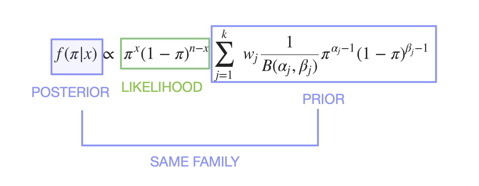
Beta Prior is a conjugate to the Posterior. Merriam-Webster Dictionary on “conjugate” : coupled, connected, or related.
Detour : Polack et al (2020), Phase III trial
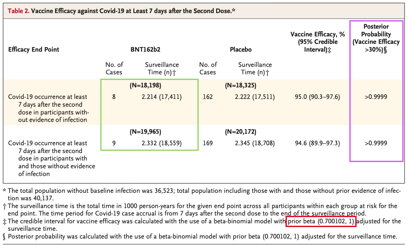
Beta Prior and Mean for BNT162b2 Phase III :

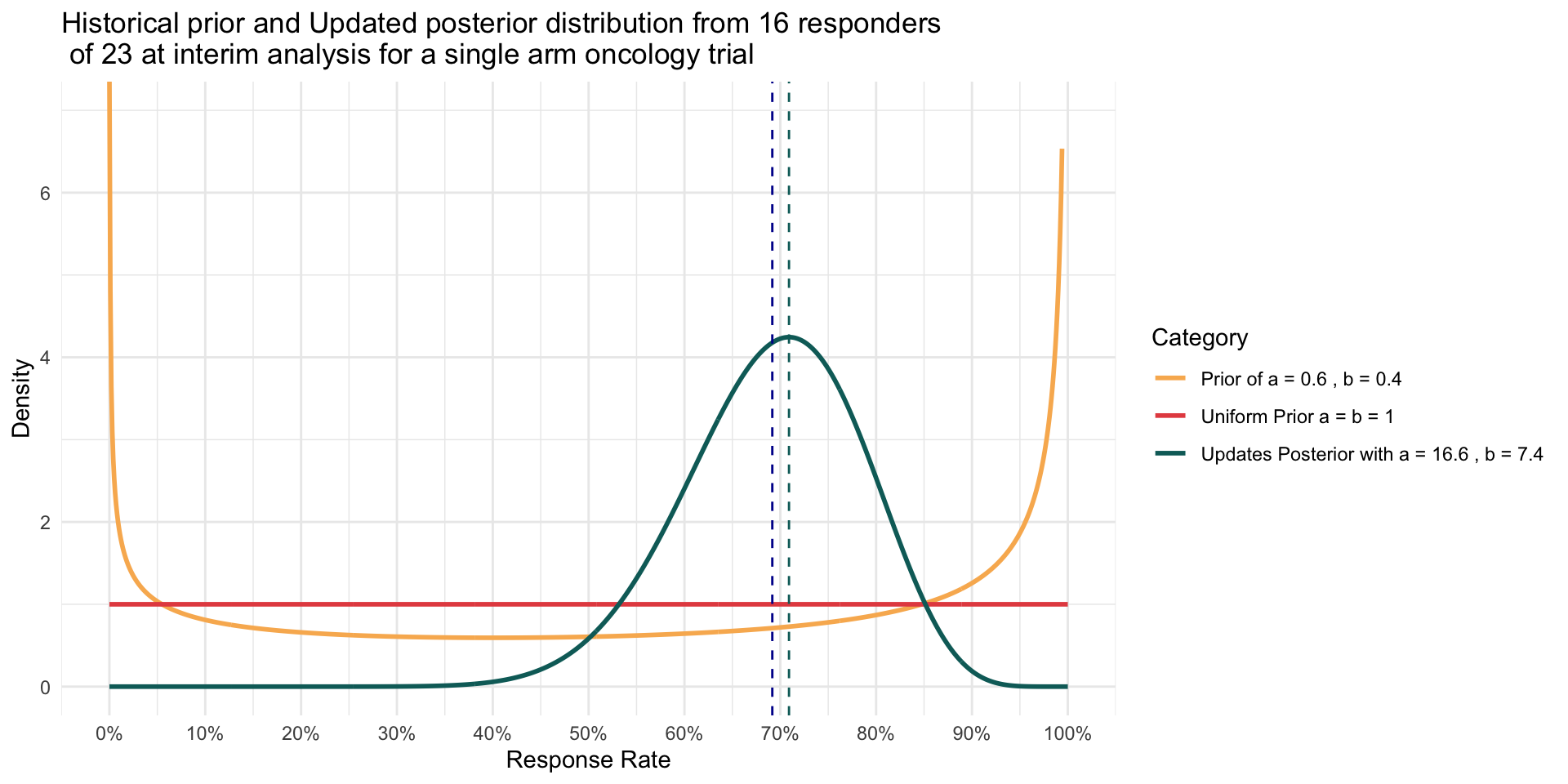
Updating the Posterior
Using the formula for the mean, where \(\alpha = 0.6, \beta = 0.4\) and at interim x = 16, n = 23 : \[ \pi = \ \frac {\alpha}{\alpha + \beta} = \ \frac {\alpha_{updated} }{\alpha_{updated} + \beta_{updated}} = \ \frac {16.6 }{16.6 + 7.4} ≈ 69.17 \% \]
\[ mode (\pi) = \ \frac {\alpha_{updated} -1 }{\alpha_{updated} + \beta_{updated} - 2} = \ \frac {16.6 -1 }{16.6 + 7.4 - 2} ≈ 70.90 \% \]
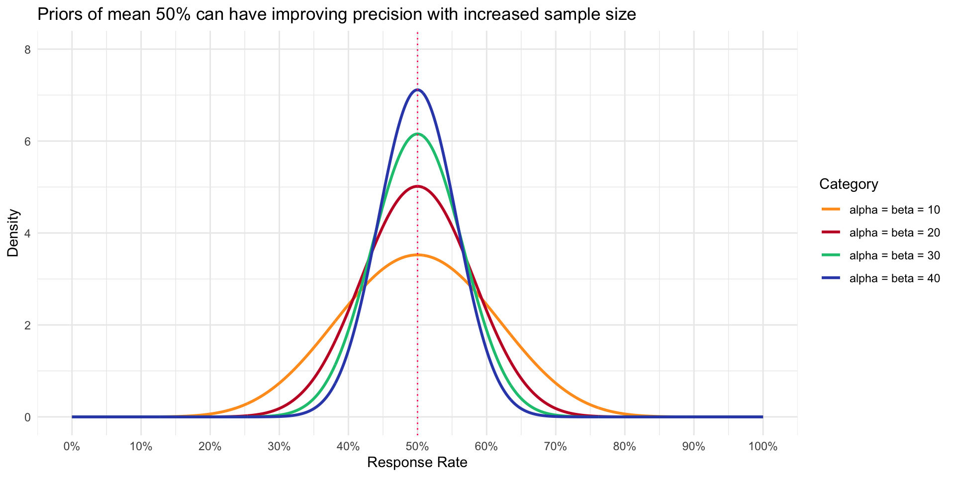
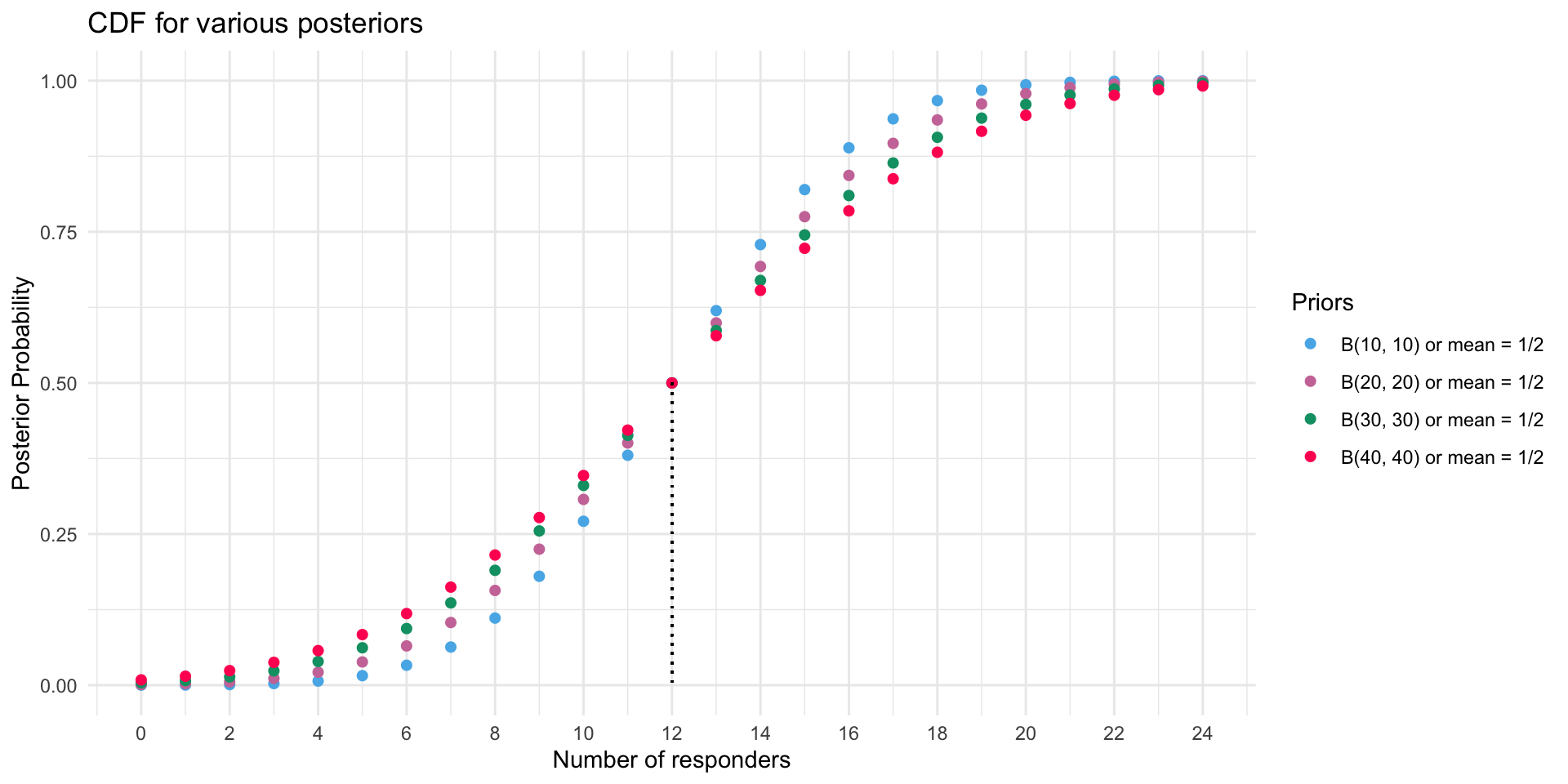
A variety of Priors
- To illustrate how density of Prior changes with increased sample size even though mean is the same
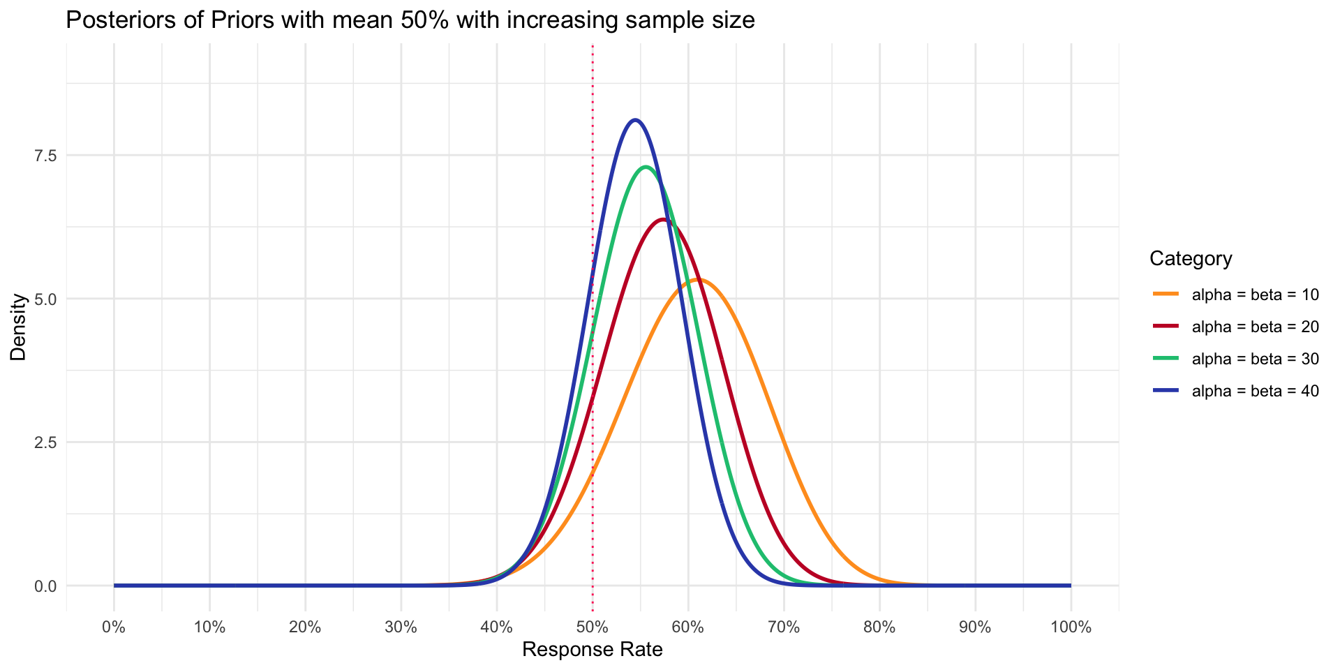
A variety of Posteriors with “different” data
- Data showed 16 of 23 responders (~69% response rate)
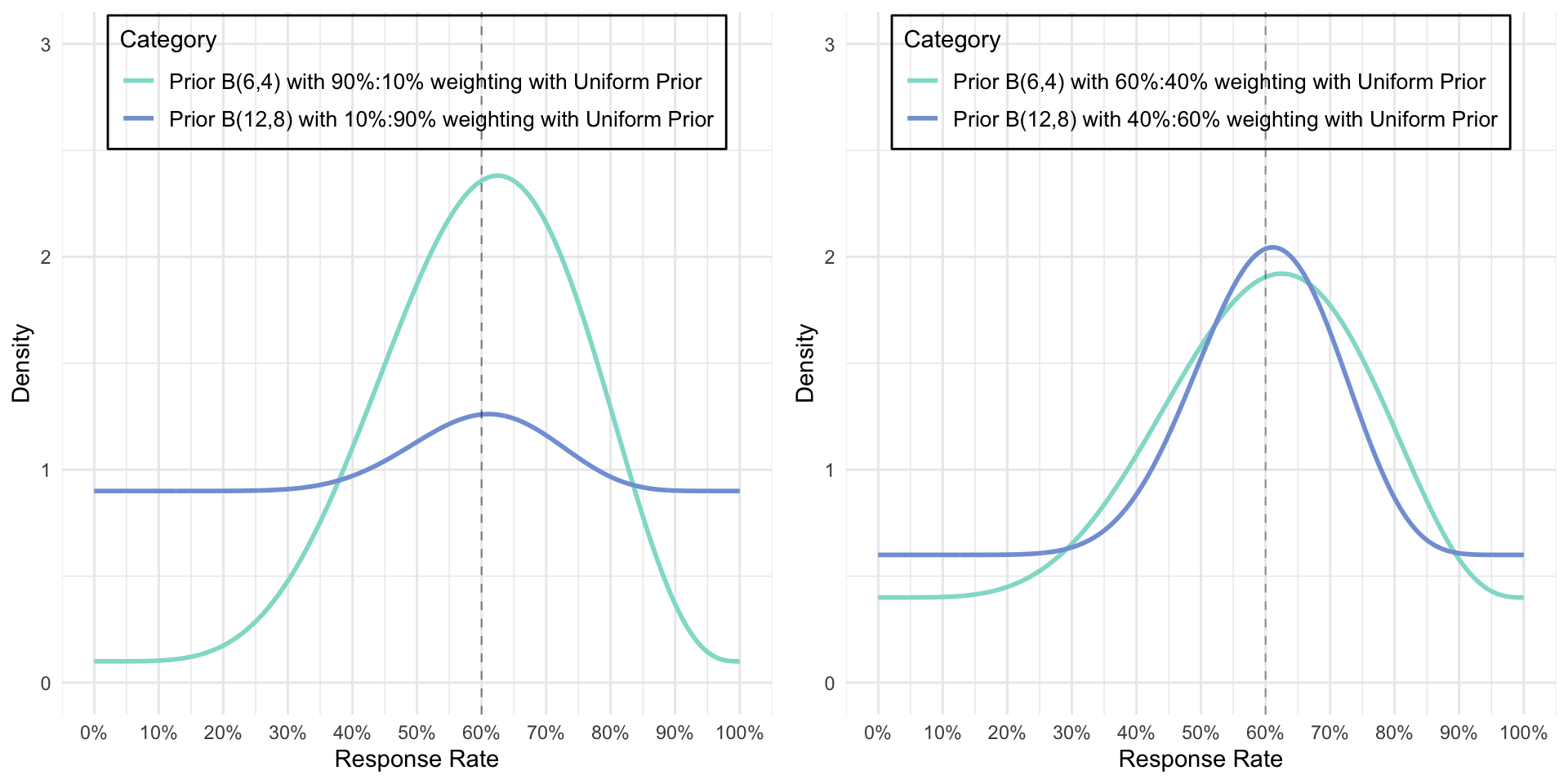
Effect of weights (and beta Mixtures)
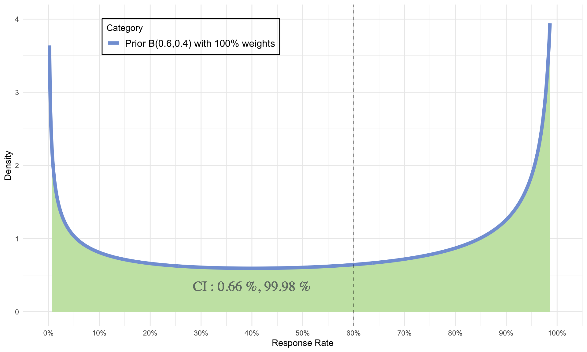
Choice of Weak Priors
- \(\alpha\) = 0.6 = number of responses
- \(\beta\) = 0.4 = number of non-responses
- \(\alpha + \beta\) = 1 = sample size
- \(\mu = 60 \%, CI = 0.66 \% \ and \ 99.98 \%\)
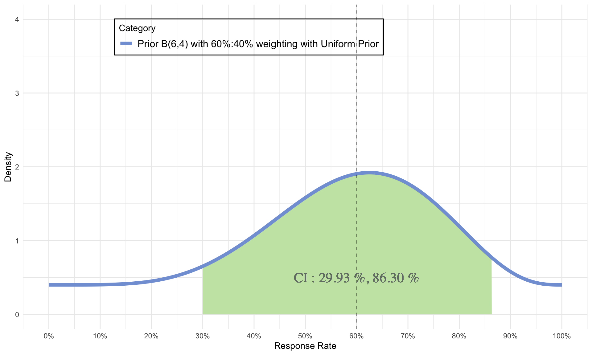
Choice of Stronger Priors
- \(\alpha\) = 6 = number of responses
- \(\beta\) = 4 = number of non-responses
- \(\alpha + \beta\) = 10 = sample size
- \(\mu = 60 \%, CI = 29.93 \% \ and \ 86.30 \%\)
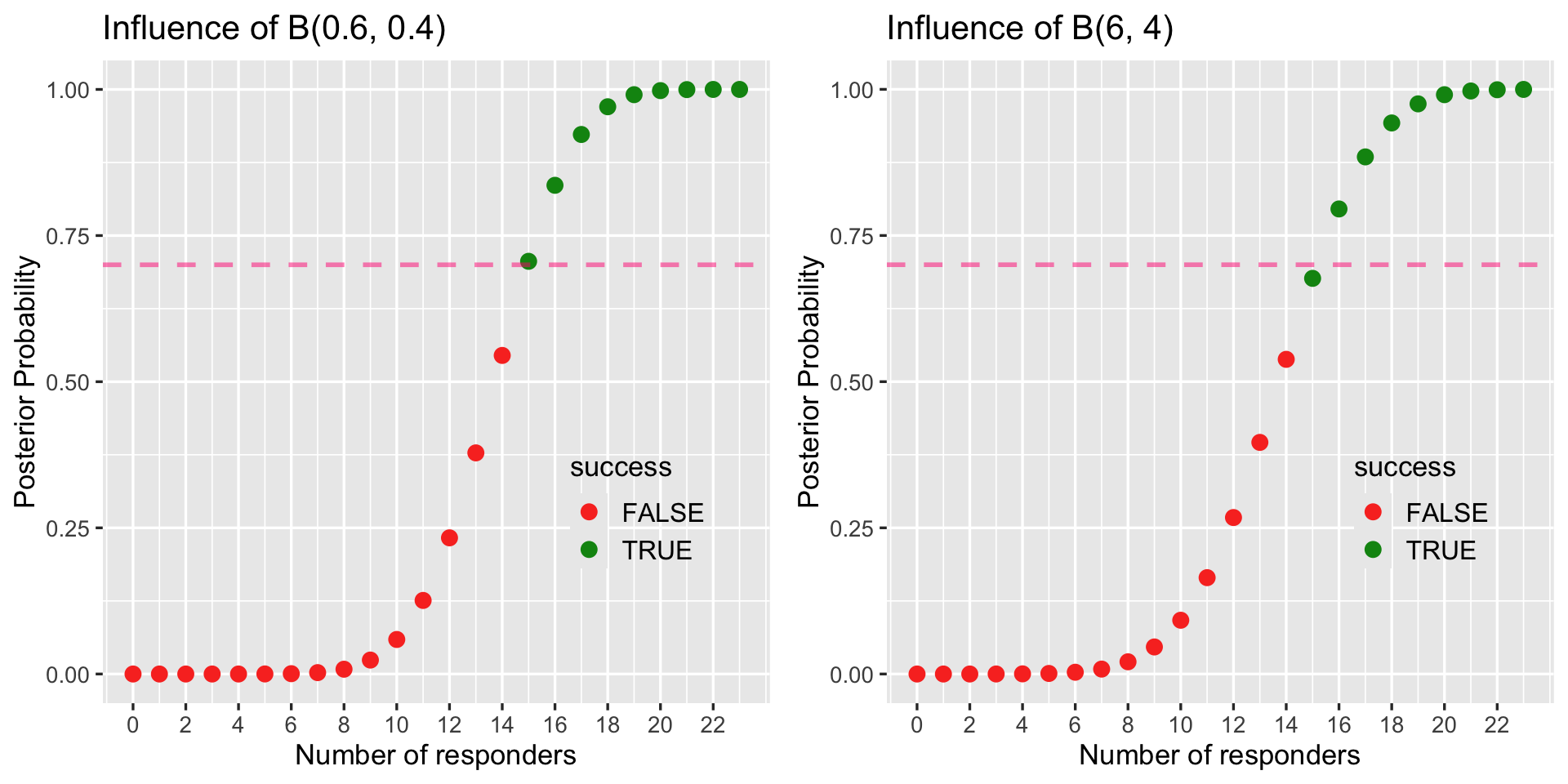
Posterior Probability
- Interim trial is efficacious if posterior probability exceeds 70% or P( RR ≥ 60 % | data ) > 70%
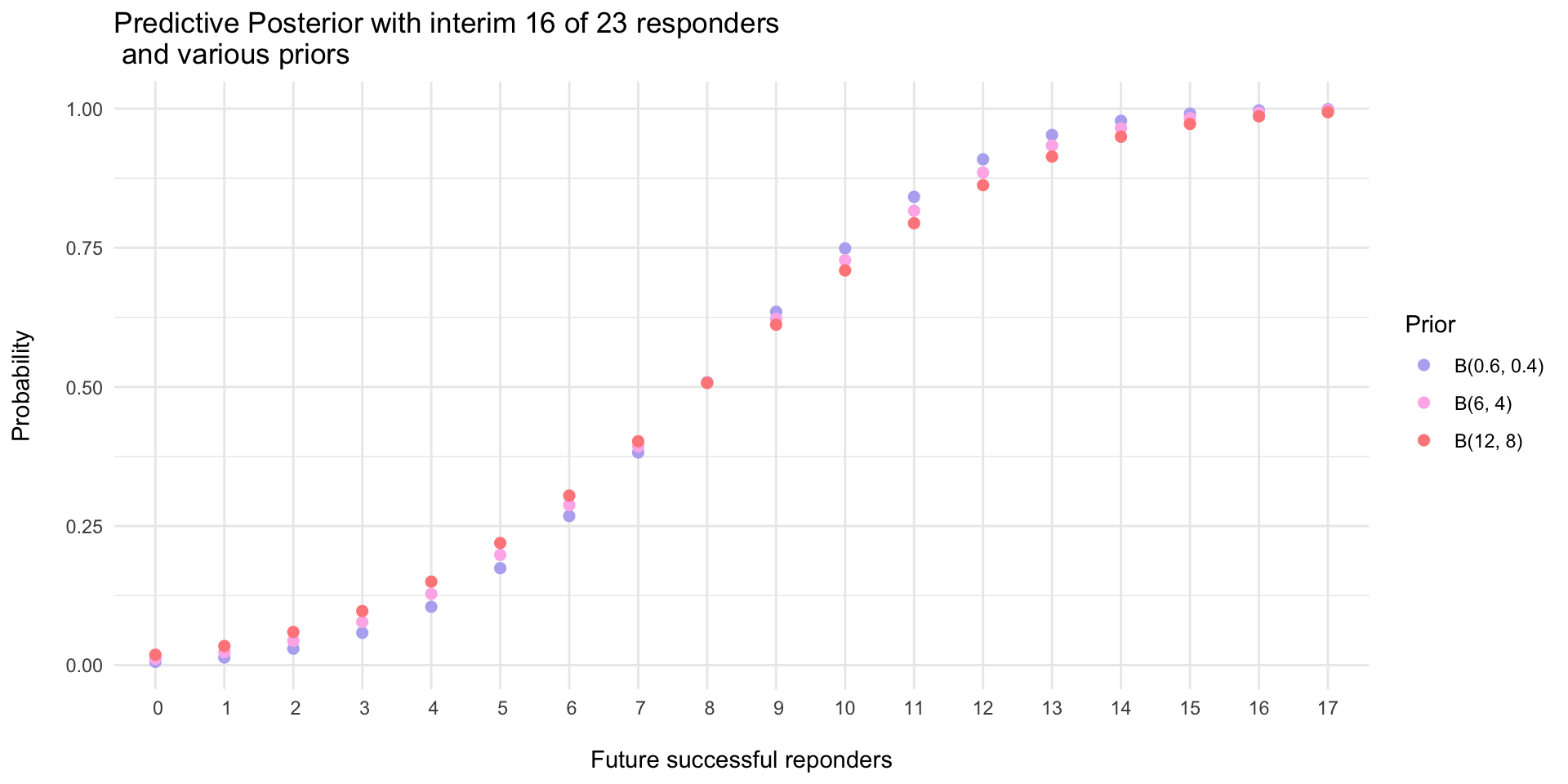
Predictive Posterior Probability
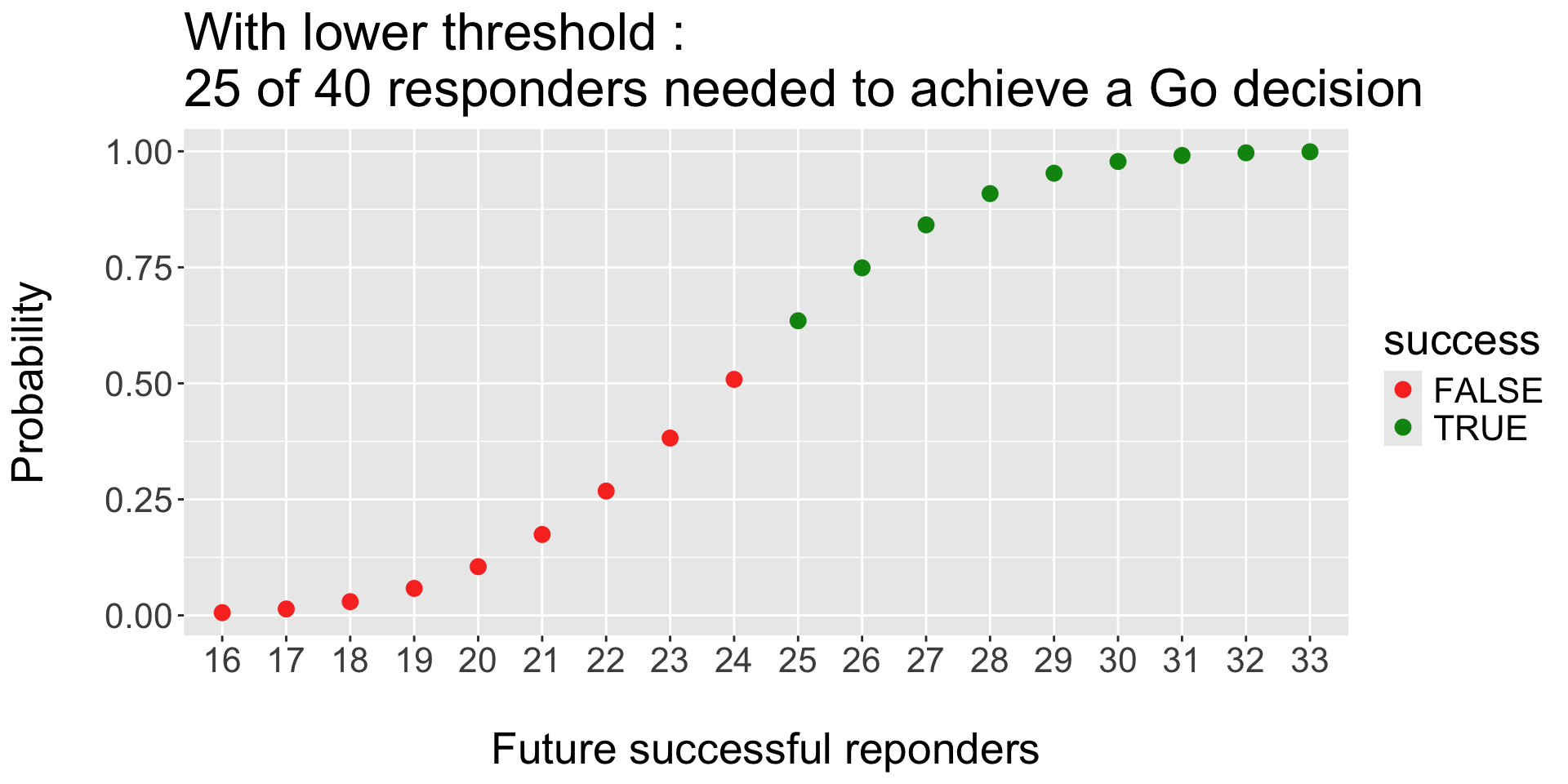
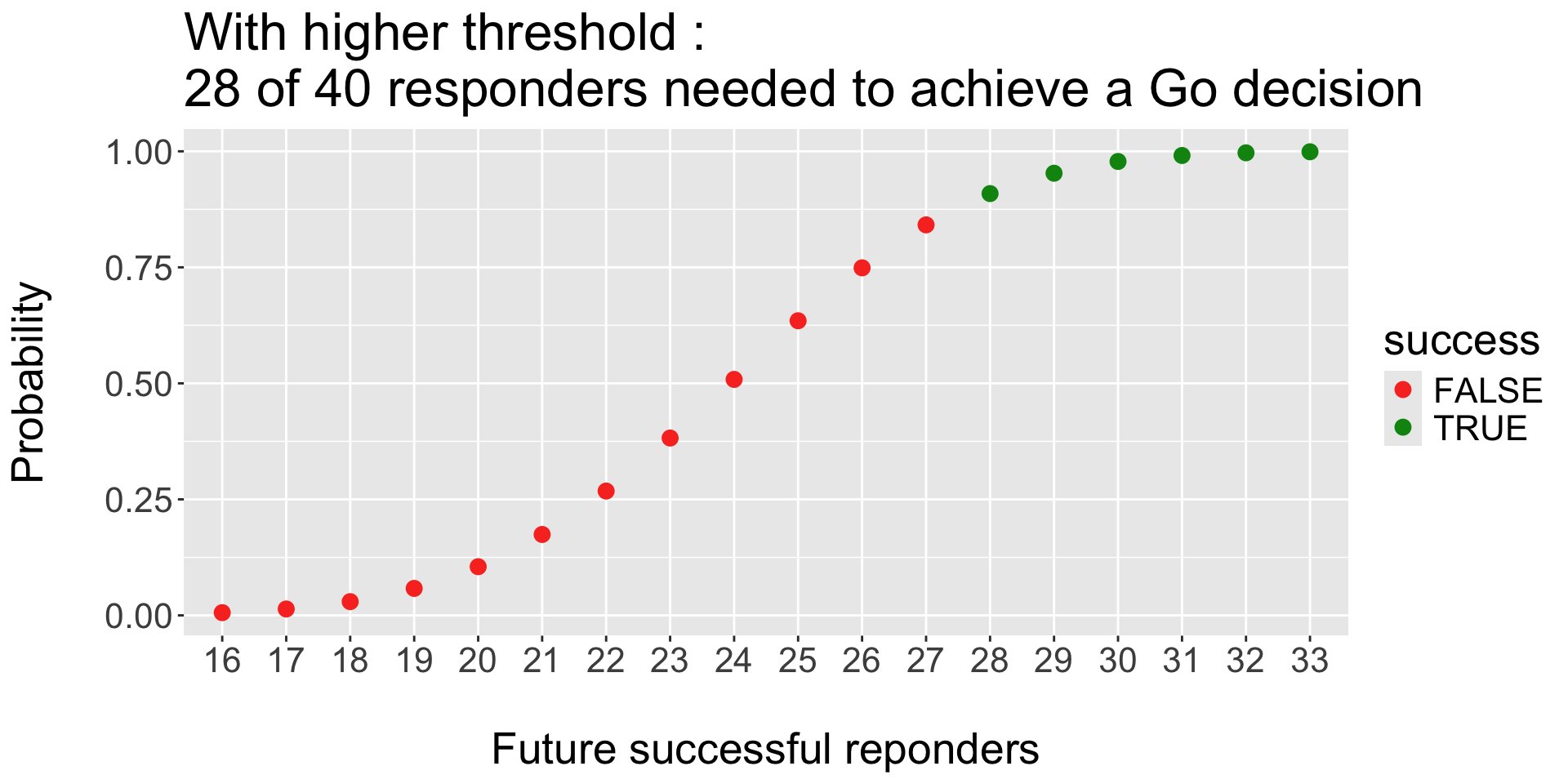
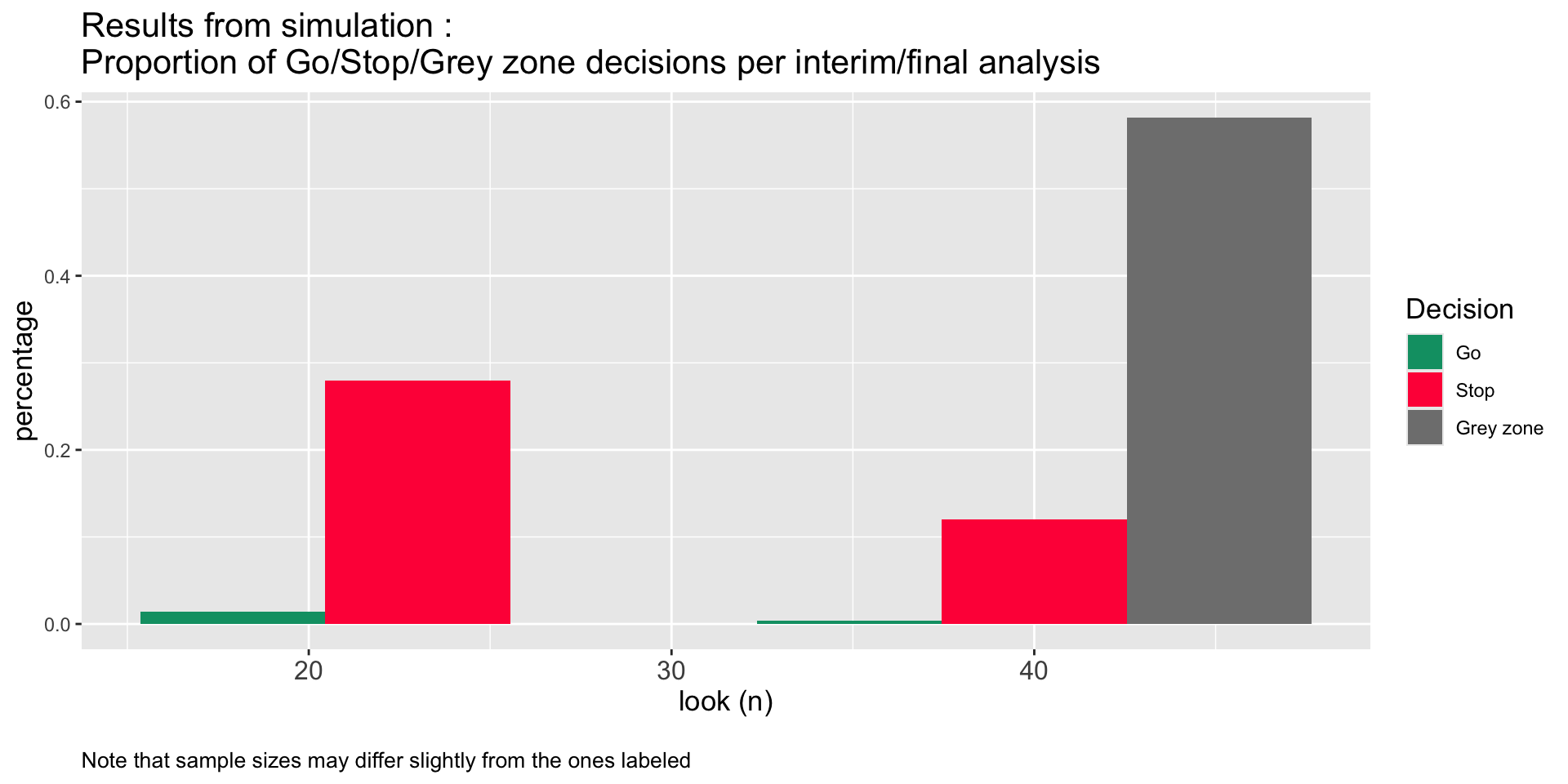
Operating Characteristics : threshold for Success (and failure):
- Efficacy criteria, e.g. we would stop for Efficacy if :
Pr( RR > p1) > tU
- Futility criteria, eg. we would stop for Futility if :
Pr( RR < p0) > tL
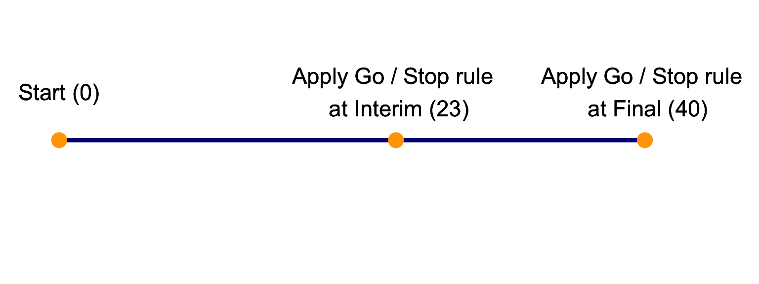
Plotting results form ocPostprob()
Concluding remarks

phase1b can be helpful to many therapeutic areas that use binary endpoint if beta priors are appropriate
Big thank you to Daniel Sabanés Bové for mentorship. Roche colleagues Isaac Gravestock, John Kirkpatrick, Craig Gower-Paige et al who collaborated and supported.
License info
Please acknowledge authors and creators

Strength of Priors (CDF version)
Strength of Priors on Predictive Posteriors (CDF version)
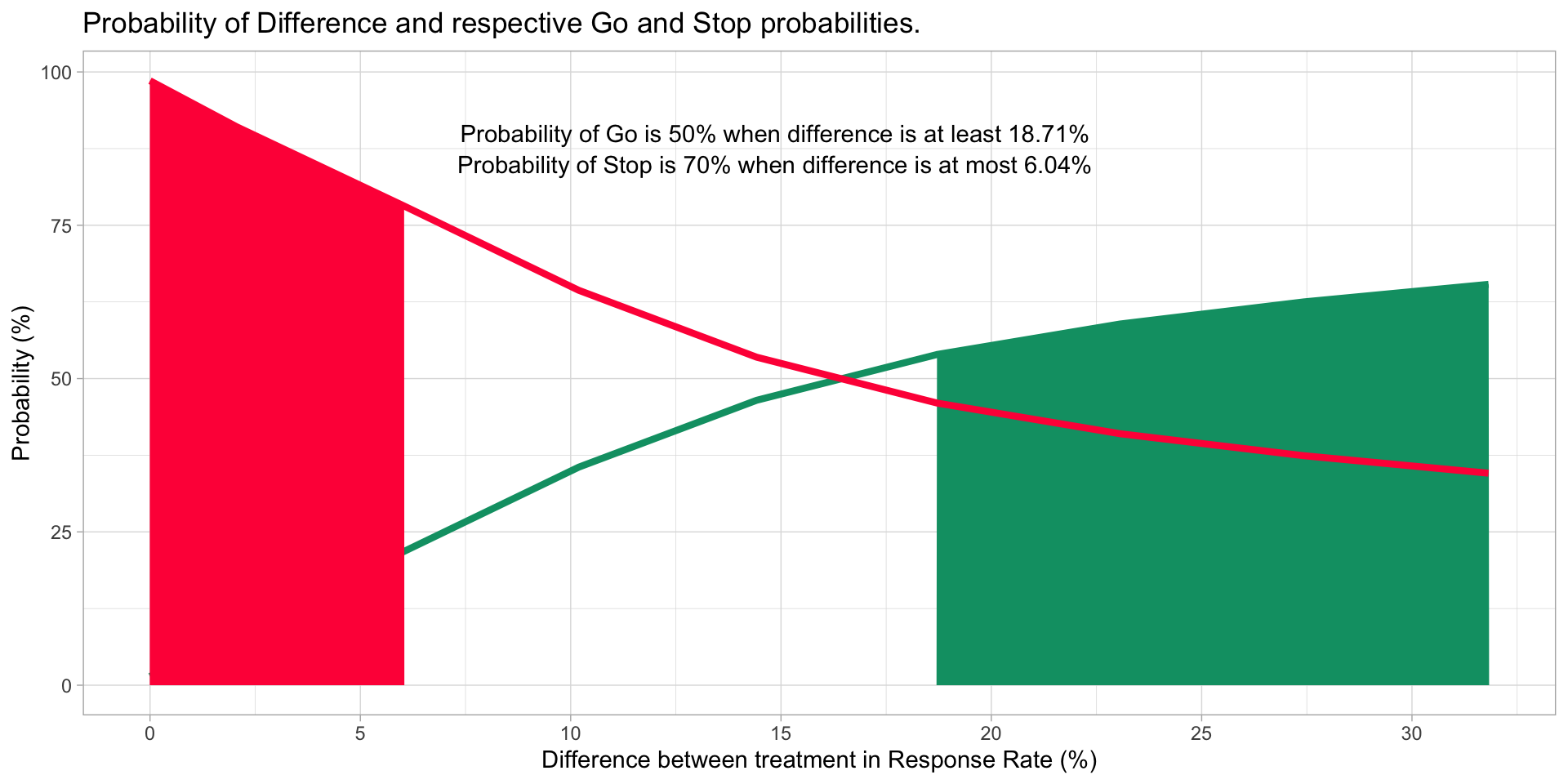
Evaluating the difference between two arms ?
Meaningful improvement if \[ \Delta > 15\% \ when \ \Delta = \pi_{E} - \pi_{S}\]
Efficacious if \[ Pr( \Delta > 15 \% | data ) > 70\% \ otherwise \ Pr( \Delta < 15 \% | data ) > 70\% \]