── R CMD build ─────────────────────────────────────────────────────────────────
* checking for file ‘/private/var/folders/36/1t9xtfl51px173qfsbg8tlcc0000gn/T/RtmpQWrj7e/remotes91b72c122d24/Genentech-phase1b-617e6f9/DESCRIPTION’ ... OK
* preparing ‘phase1b’:
* checking DESCRIPTION meta-information ... OK
* checking for LF line-endings in source and make files and shell scripts
* checking for empty or unneeded directories
* building ‘phase1b_1.0.0.tar.gz’
Warning in utils::tar(filepath, pkgname, compression = compression, compression_level = 9L,  :
  storing paths of more than 100 bytes is not portable:
  ‘phase1b/tests/testthat/_snaps/plotBetaDiff/plot-of-distibution-of-difference-of-two-arms-with-beta-mixture.svg’
Warning in utils::tar(filepath, pkgname, compression = compression, compression_level = 9L,  :
  storing paths of more than 100 bytes is not portable:
  ‘phase1b/tests/testthat/_snaps/plotOc/plot-of-simulation-result-for-single-arm-posterior-predictive-probability.svg’
Warning in utils::tar(filepath, pkgname, compression = compression, compression_level = 9L,  :
  storing paths of more than 100 bytes is not portable:
  ‘phase1b/tests/testthat/_snaps/plotOc/plot-of-simulation-result-for-single-arm-posterior-probability.svg’
Warning in utils::tar(filepath, pkgname, compression = compression, compression_level = 9L,  :
  storing paths of more than 100 bytes is not portable:
  ‘phase1b/tests/testthat/_snaps/plotOc/plot-of-simulation-result-with-relativedelta-for-posterior-predictive-probability.svg’
Warning in utils::tar(filepath, pkgname, compression = compression, compression_level = 9L,  :
  storing paths of more than 100 bytes is not portable:
  ‘phase1b/tests/testthat/_snaps/plotOc/plot-of-simulation-result-without-relativedelta-for-posterior-predictive-probability.svg’

Practical Bayesian Statistics

Audrey Yeo
Thursday, March 27
08:00
DAGStat 2025
Berlin, Germany

Practical Bayesian Statistics?

A gentle refresher on probability theory, Bayesian Framework and Intuition for effective application in Biostatistics

• Build a simple Bayesian Model
  • Test out different Priors
  • Infer from different Posteriors
• Discussing ideas for your own work

Agenda

What’s covered

• Proper Priors
• Discrete endpoints
• Credible Interval
• Posterior Probability
• Predictive Posterior Probability
• if time permits, discussion on example applications

What’s not covered

• Improper Priors
• Continuous endpoints
• Complex simulation
• Comparison with hypothesis testing using Bayes Factors

Intro myself

Intro myself

Career

• joined R & D at Roche in mid 2022 :

  • Biostats Lead in Early Oncology Trials
  • Study Statistician for phase I-II, phase III trials
  • Led Roche/Genentech Dose Escalation on new SCE
  • Led the development of R package phase1b
  • Instructor for Julia Course Basel (Data Science, Quarto, ML modules)
  • Co-organiser and Presenter many Methodology seminars

• phase1b’s world debut in 2024 :

  • PSI 2024
  • useR!2024
  • R/Pharma 2024
  • Effective Statistician conference
  • BMS, UBC, Roche/ Genentech

A starting example

\[P( awake\ | \ coffee ) \]

\[P( awake \ | \ coffee + enthusiasm )\]

\[P( awake \ | \ coffee + enthusiasm + breakfast )\]

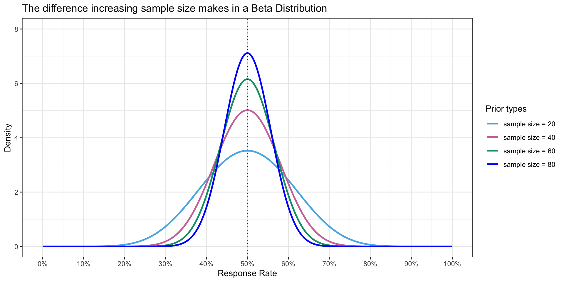
Everything is a distribution

Upon visual inspection, increase sample sizes leads to

• Better precision
  • Estimates and Credible Interval are more precise

These are benefits of the Bayesian paradigm

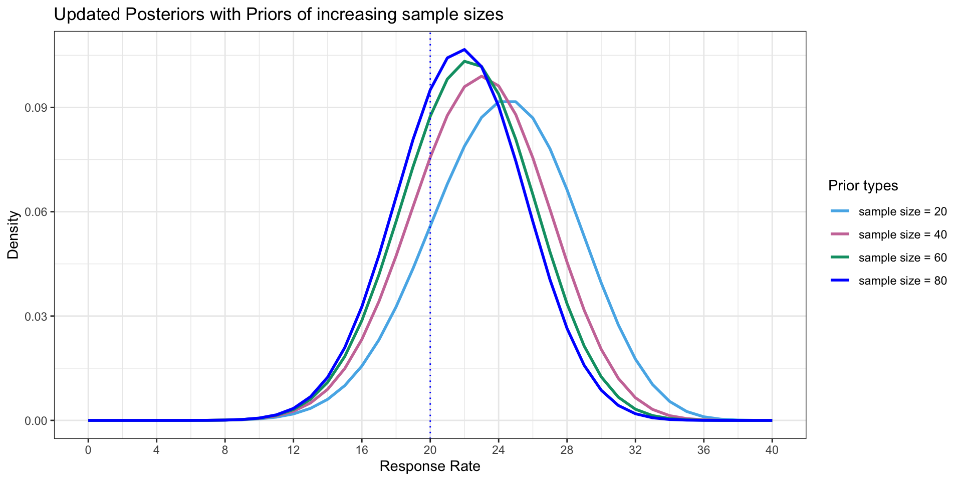
Using priors to improve precision

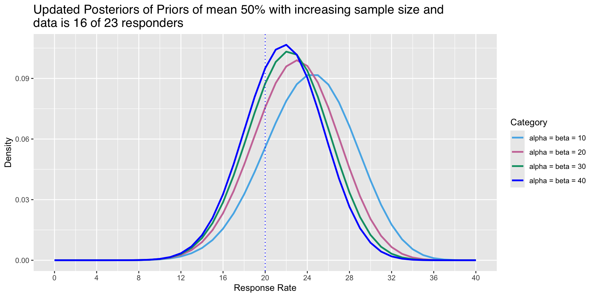
• Priors that incorporate higher \(\alpha\) and \(\beta\) parameters influence the posterior, given data stays the same (16 / 23 responders in likelihood)

Quiz

1. Increased sample size in prior information can improve precision of credible intervals

• TRUE
• FALSE

Different Perspective : neither are wrong

Example	Frequentist	Bayesian
\(\theta\)	Known and fixed according to some distribution	A random variable we can infer from some distribution
Model or Distribution	Build a model, e.g. Likelihood using data	P(\(\theta\) | data, prior )
Method	OLS, Maximum Likelihood	prior multiplied by likelihood
Inference	via hypothesis testing	P(\(\theta\) > \(\theta_{c}\) | data, prior )
What is the probability of a fair coin toss ?	Since we toss this n times, it would converge to 0.5	it’s 0 or 1

A Bayesian model looks like the Bayes Thereom or Bayes Rule

For Event A and B :

\[ 0 < P(A) < 1\]

\[ P(B) > 0\] \[ {P( B | A)} = { {P(A|B)P(B)} \over {P(A) } } \] Law of Total probability

\[P(A) = \sum_{i=1}^{n} P(A \cap B_i)\]

Using the definition of conditional probability, we can rewrite this as:

\[P(A) = \sum_{i=1}^{n} P(A | B_i) P(B_i)\] \[ P(A) = \sum_{i=1}^{n} P(A \cap B_i) = \sum_{i=1}^{n} P(A | B_i) P(B_i)\]

\[P(A) = P(A | B_1) P(B_1) + P(A | B_2) P(B_2) + P(A | B_3) P(B_3)\]

Motivating example for Biostatistics

\[ Sensitivity = P(T^{+} \ | \ D^{+} \ ) = True \ Positive \ rate \] \[ Specificity = P(T^{-} \ | \ D^{-} \ ) = True \ Negative \ rate \] \[ 1 - Sensitivity = P( T^{-} \ | \ D^{+} \ ) = False \ Negative \ rate \] \[ 1- Specificity = P(T^{+} \ | \ D^{-} \ ) = False \ Positive \ rate \]

Normalising constant : 1 less worry in your life

\[ P(A|B) = { {P(B | A) P (A)} \over { P(B)} } \] \[ P(A|B) = {P(B | A) \over P(B) } + {P (A) \over P(B) } \] \[ P(A|B)*P(B) = {{P(B | A)}} * { P (A)} \]

Demonstration only : Law of Total Probability

\[ P(B) = 1 = P(B|A_1)P(A_1) + P(B|A_2)P(A_2) + P(B|A_3)P(A_3) \] \[ P(A|B)*1 = P(B | A) + P (A) \]

\[ Posterior \ \propto \ Likelihood \ Prior\]

Let’s look at a Biostatistics example

Biostatistics solution I

Biostatistics solution II

Common use of Bayesian Statistics

1. SARS-CoV2 Diagnostic tests

2. Modeling transmission mechanism to infer treatment efficacy of different drugs and combination therapy against Trichuris trichiura by Grolimund et al (2024)

As an example, we elaborate on 2.

Modeling Egg Counts:

\[Y_{i_{jgds}}^{(0)} \sim NB(\mu_{i_{jgd}}^{(0)}, k^{(0)})\]

At baseline, egg counts are assumed to follow a negative binomial distribution. ::: {.column width=“15%”}

Mean \(\mu\) egg count was modeled by the gamma distribution.

\[ \mu \sim \ Gamma ( \mu_{jg}^{0}, \sigma_{jg}^{0}, \sigma_{jg}^{0} ) \]

The parameters used for the gamma distribution were:

• For \(\mu_{jg}^{(0)}\) (mean egg count): a gamma distribution with a mean of 50 and a variance of 1250

• For \(\sigma_{jg}^{(0)}\) (standard deviation of egg count): an exponential distribution with a mean of 0.5 and a variance of 0.25.

• For \(\sigma_{jg}^{(0)}\) a gamma distribution with mean 1 and variance 1

::::

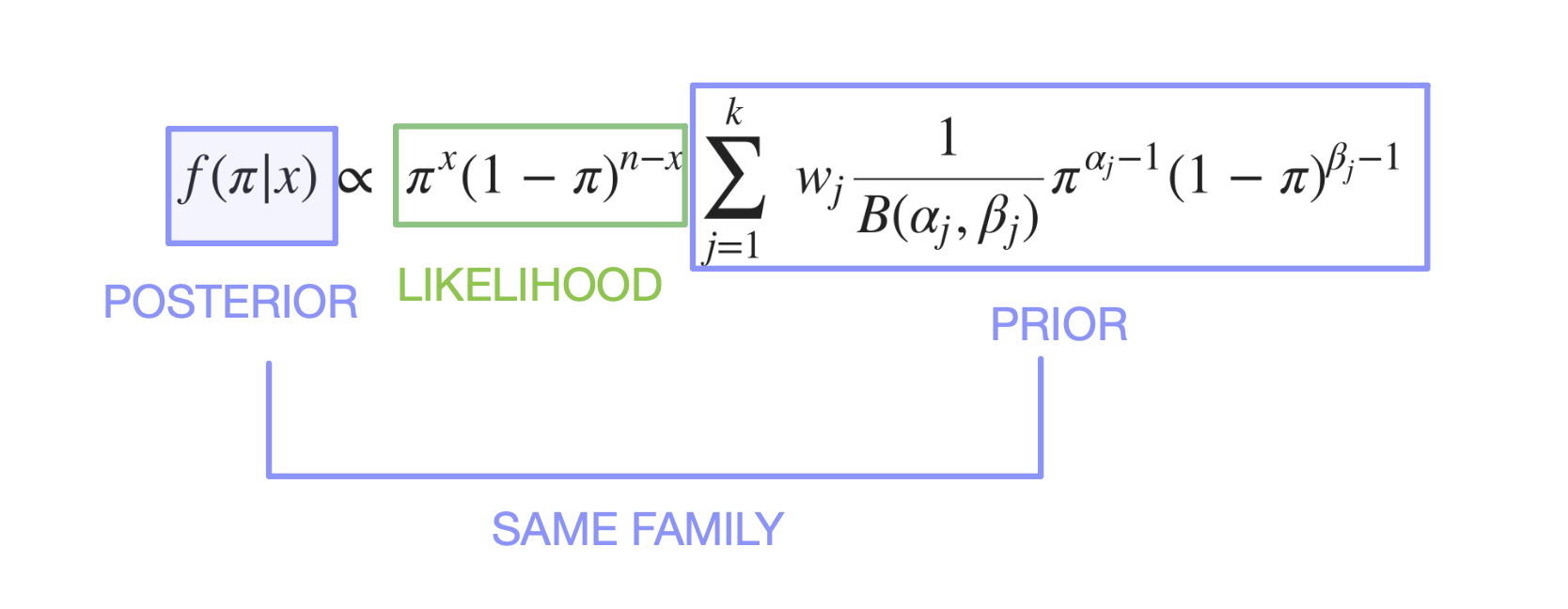
The Conjugate Prior

Merriam-Webster Dictionary on “conjugate” : coupled, connected, or related.

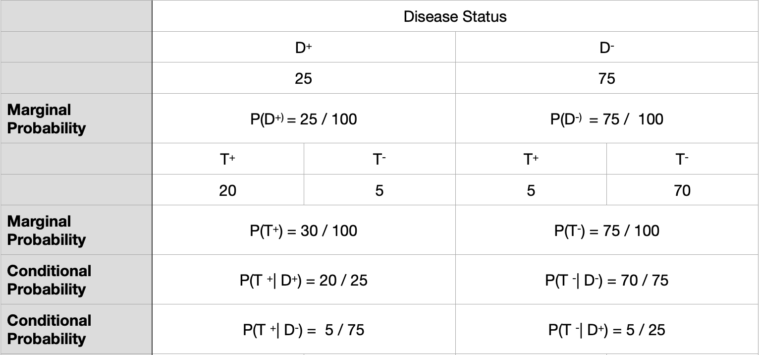
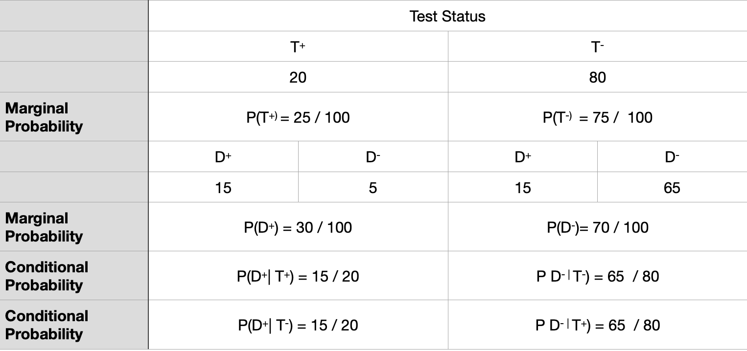
\[ {P( B | A)} = { {P(A|B)P(B)} \over {P(A) } } \]

Choices

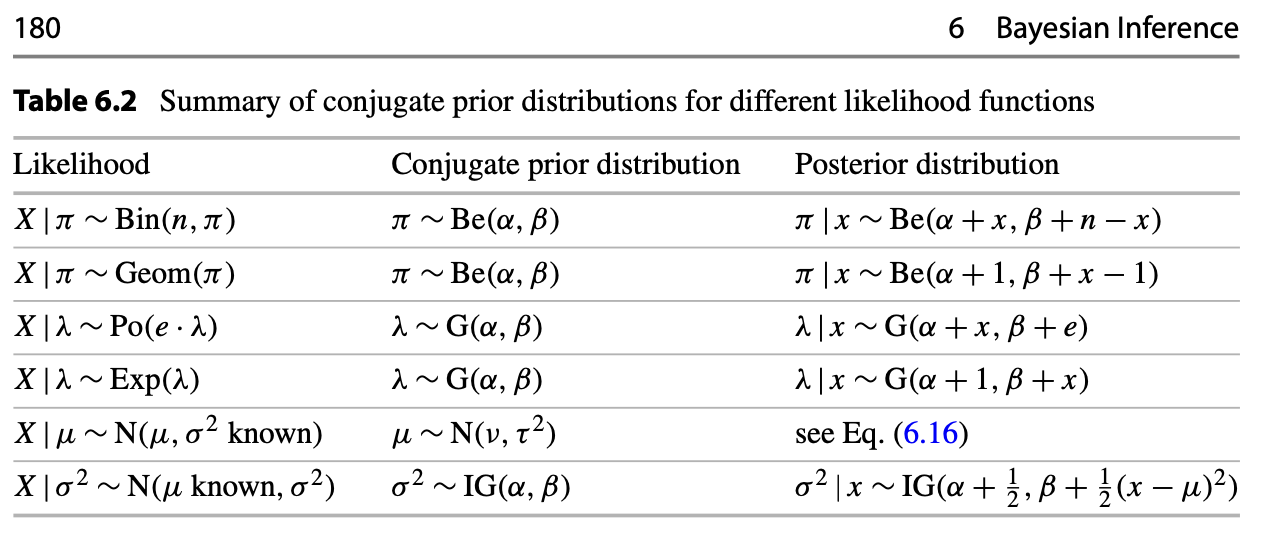
Summary table from Likelihood and Bayesian Inference from Held & Sabanés Bové (2020)

Quiz 2

\(\pi\) or Response Rate can be modeled by the Beta Distribution

• TRUE

• FALSE

About phase1b

• 2015 : Started as a need in Roche’s early development group, package development led by Daniel Sabanés Bové in 2015.

• 2023 : Refactoring, Renaming, adding Unit and Integration tests as current State-of-Art Software Engineering practice.

• 100% written in R and Open Source.

• website : genentech.github.io/phase1b/

library(devtools)
devtools::install_github("https://github.com/Genentech/phase1b")
library(phase1b)

Use case:

A single arm novel therapeutic with an assumed control response rate is at most 60%

Example	Interim	Final
Responders	16	23
n	23	40
Response rate	69.57 %	57.5 %
Posterior probability*	ask phase1b	ask phase1b
Predictive posterior probability*	ask phase1b	-
Decision to develop molecule further : Go/Stop/Grey Zone	ask phase1b	ask phase1b

Prior and Posterior of Beta Distribution for \(\pi\)

• Conjugate Prior is \(f(\pi)\), where \(\pi \sim {Beta(\alpha, \beta)}\), same family of distribution of Posterior
• We know the mean response rate (RR) is : \[\pi = \ \frac {\alpha}{\alpha + \beta}\]
• Likelihood is \(f(x|\pi)\), where \(x \sim {Binomial(x, n)}\)

• The updated Posterior \(f( \pi | x )\) is again a \(Beta\) distribution (same family as prior) : \[ \pi| \ x \sim Beta(\alpha + x, \ \beta + n - x)\] where \(x\) is the number of responders of current trial
• Posterior Probability :
  \(P (\pi > 60 \% | \alpha + x, \beta + n - x )\)
• Predictive Posterior Probability :
  \(P (success \ or \ failure \ at \ final)\)

try it yourself :

Parameters:

• Historical trial showed result of 1 of 3 responders
• we then set alpha = 1, beta = 2
• expected mean for prior distribution = 1 / 1 + 2
• Current experiment has 16 / 23 responders
• expected mean for posterior distribution = 1 + 16 / 17 + 2 + 23 - 16
  • this mean is 17 / 17 + 9 ≈ 65 %

example_alpha = 1
example_beta = 2
phase1b::plotBeta(alpha = example_alpha + x, beta = example_beta + n - x)

Quiz 3

The expected value of mean in the Beta Distribution is/are :

• \[ \mu = {{\alpha} \over {\alpha + \beta }}\]

• \[ \mu = {{\alpha + x} \over {\alpha + \beta }}\]

• \[ \mu = {{\alpha_{updated}} \over {\alpha_{updated} + \beta_{updated} }}\]

Posterior formulation :

\[ f(\pi | x) \propto \ \pi^{x} (1-\pi)^{n-x} * \frac {1}{B(\alpha, \beta)} \pi^{\alpha-1}(1-\pi)^{\beta-1} \]

• (weighted sum version)

\[ f(\pi | x) \propto \ \pi^{x} (1-\pi)^{n-x} * \sum_{j = 1}^{k} \ w_j \frac {1}{B(\alpha_j, \beta_j)} \pi^{\alpha_j-1}(1-\pi)^{\beta_j-1} \]

Updating the Posterior

Using the formula for the mean, mode and median, where :

• \(\alpha = 0.6, \beta = 0.4\) and

• interim x = 16, interim n = 23 :
  \[ \pi = \ \frac {\alpha}{\alpha + \beta} = \ \frac {\alpha_{updated} }{\alpha_{updated} + \beta_{updated}} = \ \frac {16.6 }{16.6 + 7.4} ≈ 69.17 \% \]

  \[ mode (\pi) = \ \frac {\alpha_{updated} -1 }{\alpha_{updated} + \beta_{updated} - 2} = \ \frac {16.6 -1 }{16.6 + 7.4 - 2} ≈ 70.90 \% \] \[ median ( \pi) ≈ \ \frac {\alpha_{updated}}{ \alpha_{updated} + \beta_{updated} - \frac{2}{3} } ≈ 69.71 \% \]

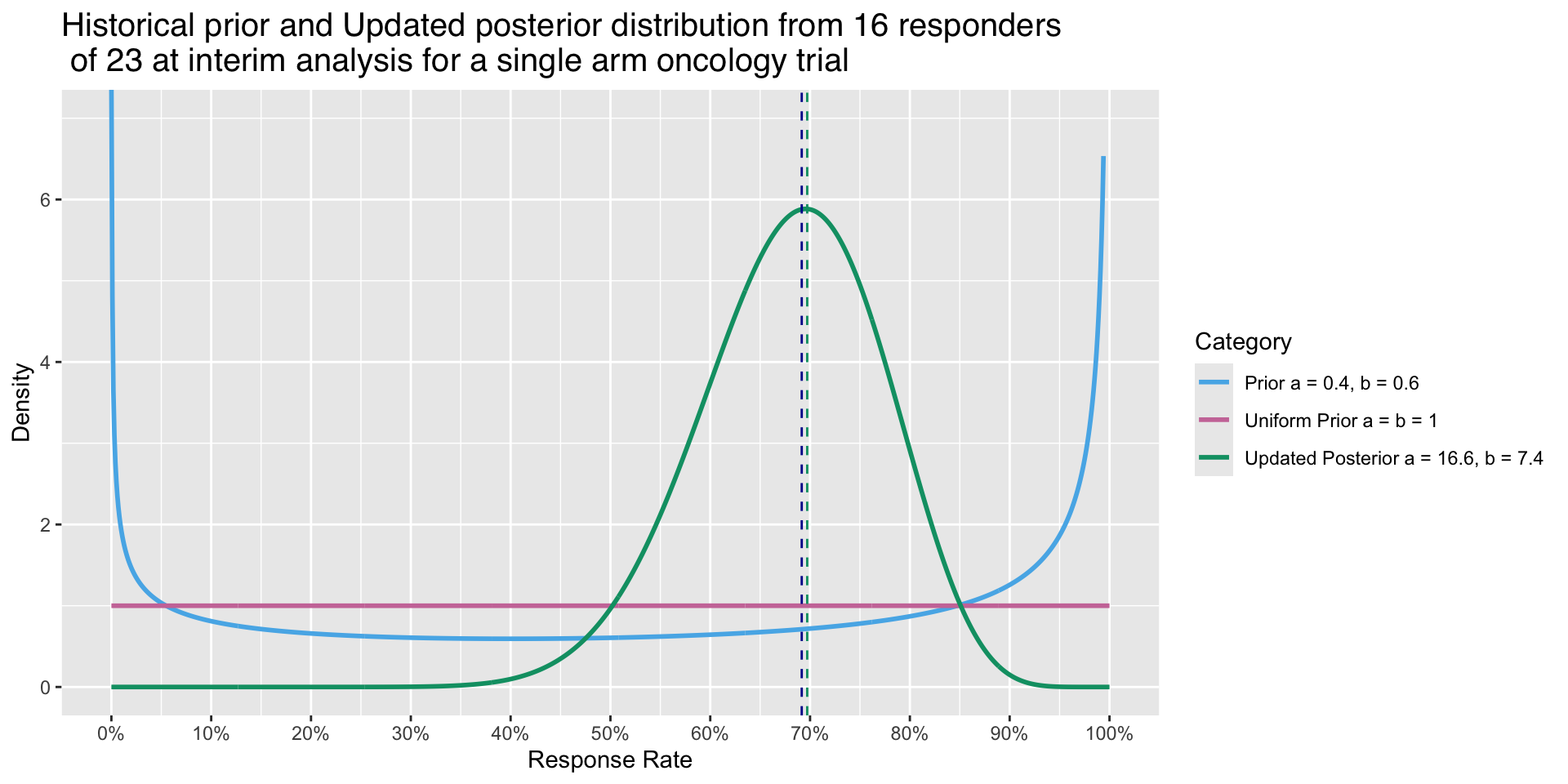
Graphical representation of the updated Posterior

• Prior parameters are \(\alpha\) = 0.6, \(\beta\) = 0.4
• Updated Posterior parameters are \(\alpha\) = 16.6 and \(\beta\) = 7.4

Effect on varying weight on different priors Example

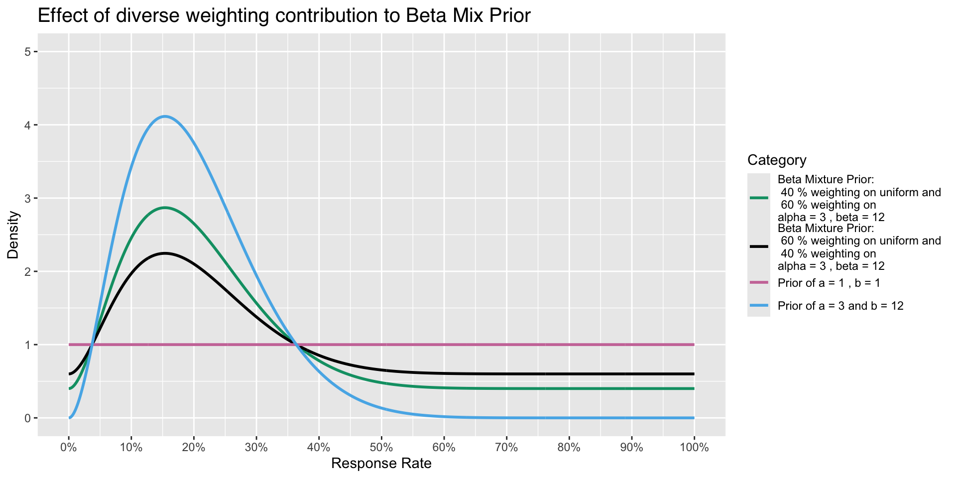
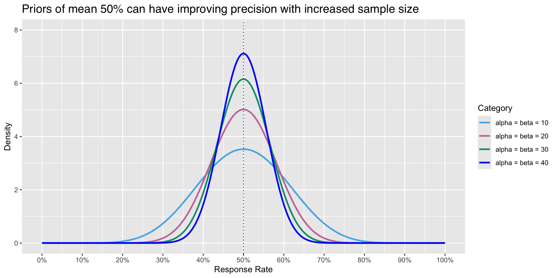
A variety of Priors

• To illustrate how density of Prior changes with increased sample size even though mean is the same

A variety of Posteriors

• To illustrate how density of Posterior changes with increased sample size even though mean is the same

postprob() example (Lee & Liu, 2008)

Example	Interim
Responders	16
n	23
Response rate	69.57 %
Standard of Care Response rate	60 %
Posterior probability	postprob( ) call from phase1b

phase1b::postprob(x = 16, n = 23, p = 0.60, par = c(0.6, 0.4))

[1] 0.8359808

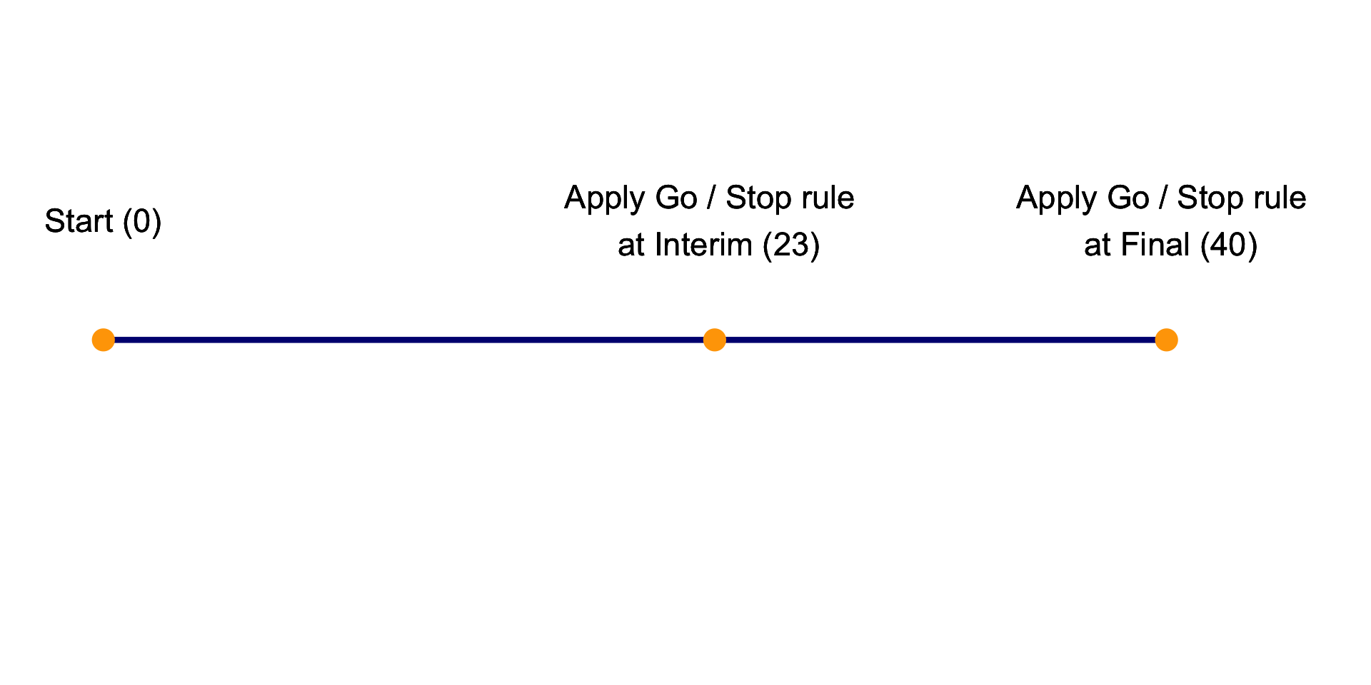
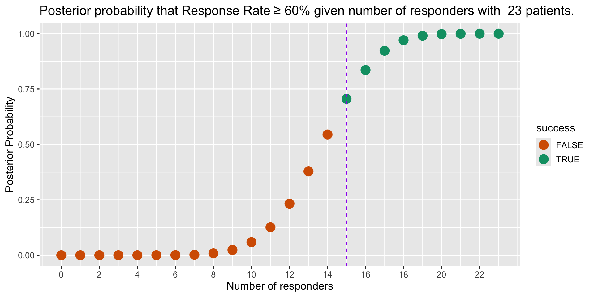
Posterior Probability

• Interim trial is efficacious if posterior probability exceeds 70% or P( RR ≥ 60 % | data ) > 70%

Figure 1

Beta prior mixture

• phase1b facilitates the flexibility of using various priors and its respective weightings:

             Prior is P_E ~ sum(weights * beta(parE[, 1], parE[, 2]))

a = phase1b::postprob(x = 16,
             n = 23,
             p = 0.60,
             parE = c(0.6, 0.4), weights = 1)

b = phase1b::postprob(x = 16,
             n = 23,
             p = 0.60,
             parE = c(2, 4), weights = 1)

0.5*(a + b)

[1] 0.7187072

phase1b::postprob(x = 16,
             n = 23,
             p = 0.60,
             parE = rbind(c(0.6, 0.4), c(2, 4)), weights = c(0.5, 0.5))

[1] 0.7406505

• Posterior formulation :

\[ f(\pi | x) \propto \ \pi^{x} (1-\pi)^{n-x}\sum_{j = 1}^{k} \ w_j \frac {1}{B(\alpha_j, \beta_j)} \pi^{\alpha_j-1}(1-\pi)^{\beta_j-1} \]

predprob() example (Lee & Liu, 2008)

Example	Interim
Responders	16
n	23
Response rate	69.57 %
Standard of Care Response rate	60 %
Predictive Posterior probability	predprob( ) call from phase1b

control = 0.6
confidence_seventy = 0.7
result <- phase1b::predprob(
  x = 16, n = 23, Nmax = 40, p = control, thetaT = confidence_seventy,
  parE = c(0.6, 0.4)
)
result$result

[1] 0.8211011

confidence_ninety = 0.9
result_high_thetaT <- phase1b::predprob(
  x = 16, n = 23, Nmax = 40, p = control, thetaT = confidence_ninety,
  parE = c(0.6, 0.4)
)
result_high_thetaT$result

[1] 0.5655589

Predictive Posterior Probability (Lee & Liu, 2017)

\[ \sum_{i = 0}^{m} P( Y = i \ | \ x ) . I\ (Prob ( P > p_{0} \ | x, Y = i) > \theta_{T}) \]

\[ = \sum_{i = 0}^{m} \{ P( Y = i \ | \ x ). I\ ( B_{i} > \theta_{T} \} = \sum_{i = 0}^{m} P( Y = i \ | \ x ) . I_{i} \]

Predictive Posterior Probability (PPP)

\[ PPP = \sum_{i = 0}^{m} \{ P( Y = i \ | \ x ). I\ ( B_{i} > \theta_{T} \} = P(RR \ at final \ > 60 \%) > 70 \% \]

# The original Lee and Liu (Table 1) example:
# Nmax = 40, x = 16, n = 23, beta(0.6,0.4) prior distribution,
# thetaT = 0.7. The control response rate is 60%:
results <- phase1b::predprob(
  x = 16, # current number of responders
  n = 23, # sample size at interim
  Nmax = 40, # max sample size
  p = 0.6, # control response rate 
  thetaT = 0.7, # confidence 
  parE = c(0.6, 0.4) # prior alpha and beta
)

print(results)

$result
[1] 0.8211011

$table
   counts cumul_counts density   posterior success
1       0           23  0.0000 0.005858397   FALSE
2       1           24  0.0000 0.013782046   FALSE
3       2           25  0.0001 0.029584325   FALSE
4       3           26  0.0006 0.058130376   FALSE
5       4           27  0.0021 0.104881818   FALSE
6       5           28  0.0058 0.174328134   FALSE
7       6           29  0.0135 0.267887754   FALSE
8       7           30  0.0276 0.382146405   FALSE
9       8           31  0.0497 0.508508727   FALSE
10      9           32  0.0794 0.634871049   FALSE
11     10           33  0.1129 0.748893301    TRUE
12     11           34  0.1426 0.841482798    TRUE
13     12           35  0.1587 0.908912106    TRUE
14     13           36  0.1532 0.952764733    TRUE
15     14           37  0.1246 0.978098514    TRUE
16     15           38  0.0811 0.991013775    TRUE
17     16           39  0.0381 0.996776597    TRUE
18     17           40  0.0099 0.999003945    TRUE

results$table$density[results$table$success == TRUE] %>% sum()

[1] 0.8211

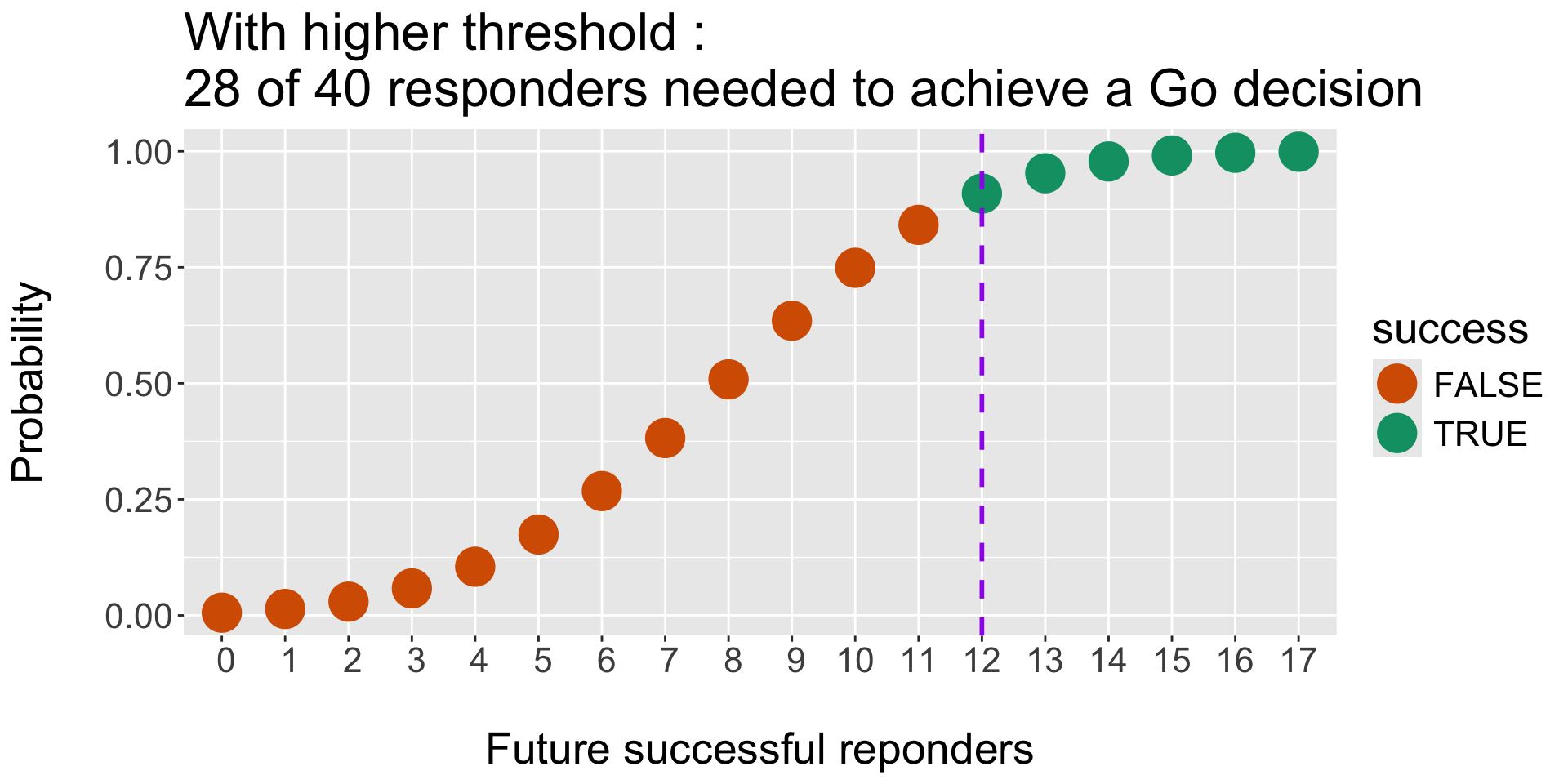
Predictive Posterior Probability

Predictive Posterior Probability is the Posterior probability of additional responders.

        (Note : 40 - 23 = 17 remaining patients. Potentially 16 + 17 responders at final = 33)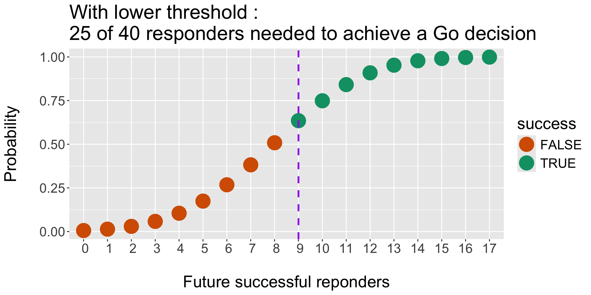

(a) \(P (\pi > 0.6 | \ data )\) > 70%

(b) \(P (\pi > 0.6 | \ data )\) > 90%

Figure 2: Predictive Posterior CDF for different Efficacy Rules

Operating Characteristics : Monte Carlo Simulations and threshold for Success (and Failure)

• Efficacy criteria, e.g. we would stop for Efficacy (Success) if : Pr( RR > p1) > tU
• Futility criteria, eg. we would stop for Futility (Failure) if : Pr( RR < p0) > tL

Rules and Operating characteristics. A use case for ocPostprob():

• Stop for Efficacy: Go if \(P( \pi > 60\% | \ data ) > 90 \%\)
• Stop for Futility: Stop if \(P( \pi < 60\% | \ data ) > 70 \%\)
• Prior of treatment arm \(Beta(0.6, 0.4)\).

set.seed(2025)
res <- phase1b::ocPostprob(
  nnE = c(23, 40), 
  truep = 0.60, 
  p0 = 0.60, 
  p1 = 0.60, 
  tL = 0.70, 
  tU = 0.90, 
  parE = c(0.6, 0.4),
  sim = 500, 
  wiggle = TRUE, 
  nnF = c(23, 40)
)

Results

ExpectedN	PrStopEarly	PrEarlyEff	PrEarlyFut	PrEfficacy	PrFutility	PrGrayZone
34	36.8 %	8.8 %	28 %	11 %	40 %	49 %

• At n = 34, we have some useful results (we did not have to evaluate 40!)

• 1/3 of results are known at interim, most of these results are in the Gray Zone

• ~ 1/2 of results are also at the Gray Zone at final

Expanded features

…. and wiggle room!

	SOC uncertainty	single-arm	two-arm	simulation	plotting	boundaries
postprob		✔️
postprobDist	✔️	✔️
predprob		✔️
predprobDist	✔️	✔️
ocPostprob		✔️		✔️
ocPostprobDist	✔️	✔️		✔️
ocPredprob		✔️		✔️
ocPredprobDist	✔️	✔️		✔️
ocRctPostprobDist	✔️	✔️	✔️	✔️
ocRctPredprobDist	✔️	✔️	✔️	✔️
plotBeta				✔️	✔️
plotDecision					✔️
plotOc					✔️
plotBounds					✔️
boundsPostprob						✔️
boundsPredprob						✔️

Some references

• Held L & Sabanés Bové D (2020) Likelihood and Bayesian Inference : Applications in Medicine and Biology, 2nd Edition.

• LeSaffre E & Lawson A (2012) Bayesian Biostatistics, First Edition,

• Thall P F, Simon R (1994), Practical Guidelines for Phase IIB Clinical Trials, Biometrics, 50, 337-349.

• Lee J J, Liu D D (2008), A Predictive probability design for phase II cancer clinical trials, 5(2), 93-106, Clinical Trials.

• Yeo, A T, Sabanés Bové D, Elze M, Pourmohamad T, Zhu J, Lymp J, Teterina A (2024). Phase1b : Calculations for decisions on Phase 1b clinical trials. R package version 1.0.0, https://genentech.github.io/phase1b

• Inclusive Speaker Orientation Linux Foundation

• Zeileis, Fisher, Hornik, Ihaka, McWhite, Murrell, Stauffer, Wilke (2020) colorspace: A Toolbox for Manipulating and Assessing Colors and Palettes. Journal of Statistical Software.

Thanks DAGStat 2025

Audrey Yeo
[email protected]
M Nursing (Sydney)
M Sci Biostats (Zürich)

   

etc

• Code for this talk
• Visit my website
• LinkedIn
• My GitHub repo